v. wind = 5 m/s
Billboard dimension
Length = 5,5 m
Width = 0,5 m
Control Volume :
Length = 50 m
Width = 15 m
top and bottom as symmetric side
first step in simulation using CFDSOF to get Total Pressure of air flow through the board. The explanation below describ how to do simulation. First, we make a boundary condition as control volume according the dimension above, makes grid that represent the dimension of billboard, set inlet and outlet that show how fluid start to flow and ends in left and right side of the control volume. Set symmetrical in top and bottom side that show the flow characteristic in further top and bottom side is unknown. Set the domain about type of flow is k-epsilon that represent the type flow of air is in turbulent flow. Set velocity inlet is 5 m/s as assumption of highest velocity may be pass the board. After that, we proccess the simulation by iteration until the condition of convergency is approached. Then show the results in vector and contour.
Figure 1. Grid of control volume that will domain of iteration
Figure 2. vector
of velocity magnitude of air flow
Figure 3. Contour velocity magnitude distribution
Figure 4. Contour of relative total pressure
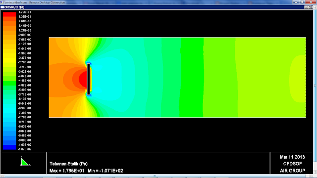
Figure 5. Contour of static pressure
After we got the results in Total pressure, we can find the forces in the surface of board by equation P = F/A, from it we can estimate bending moment value (M). In post processing CFDSOF we can see the distribution of total pressure in koordinat nodal by "lihat alfa" :
Figure 6. Relative Total Pressure distribution in grid cell
Figure 7. Table calculation to find max. bending moment
The resultan of forces is shear forces along the references point (Point 1 is the botom reference that will be attached pillar bar).
Figure 8. Shear force diagram along reference point
By integral of shear forces we get moment diagram. Total area under shear forces graph is moment diagram. We can see that bending moment max. is in point 1 reference, because in this case we use one point reference in point 1.
Figure 9. Moment diagram show max. bending moment in the reference point 1 that assumpted as bottom side of board to be fitted with pillar bar.
After we got the value for maximum bending moment (M) like showed in graph above the value is 114,075 Nm (minus signed that resultan forces is counter direction with wind direction), then we have to calculate Modulus area (W) that consists of Inertia (I) and distance of neutral axis (y).
W = I / y
As we know from the ASTM code that the material we used is carbon steel with composition and data for yield strength is Bj-52 with 3600 kg/cm2 yield strength. The material is cylinder that will we used as pillar bar for billboard.
From the data yield strength we can estimate the dimension for diameter of solid cylinder :
I = phi (D^4) / 64
by used neutral axis distance for the billboard length is 5.5 m, we used y = 5.5 m.
so, we can estimate diameter dimension by :
yield stress = Max. bending moment / Modulus area
0,36 = (114 x 5,5) / ((22/7 x D^4) / 64)
D^4 = 2,82 x 10^-5
D = 0,073 m = 7,3 cm
From calculation the formula above we can determine the dimension for solid cylinder pillar is about 0,073 m or 7,3 cm.


